Data Visualization
of Crime Inter-Alberta and within Calgary
This project is meant to vizualize crime in Calgary, and other municipalities within Alberta, Canada. Tools used were Excel, Tableau, and Jupyter Anaconda (Python).
I chose to do this project with the initial intent to see if Forest Lawn, a community in Calgary that I live in, is safe. Since then, I have refocused my intentions to have a more exploratory approach of the data set. Here are the revised questions I am most interested in answering and analyzing:
The only questions that changed from Project 1.1 were questions [4] and [6], which were originally:
I changed question [4] because it needed more detail about the level of analysis. It was unclear whether the correlations were for the city level, neighborhood level, or if it was by year or month. I since have made it clearer by specifying that it was by municipality level.
I changed question [6] because using the term "you" is very subjective. The question doesn't have a clear sense of who we're talking about and what their tolerances are, it isn't clear how a question like this can be answered. I decided to go with crime that involves drugs between Calgary, Edmonton, and Medicine Hat because I'm interested to see if drug crimes vary between these cities.
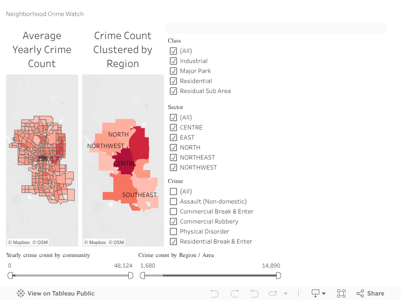
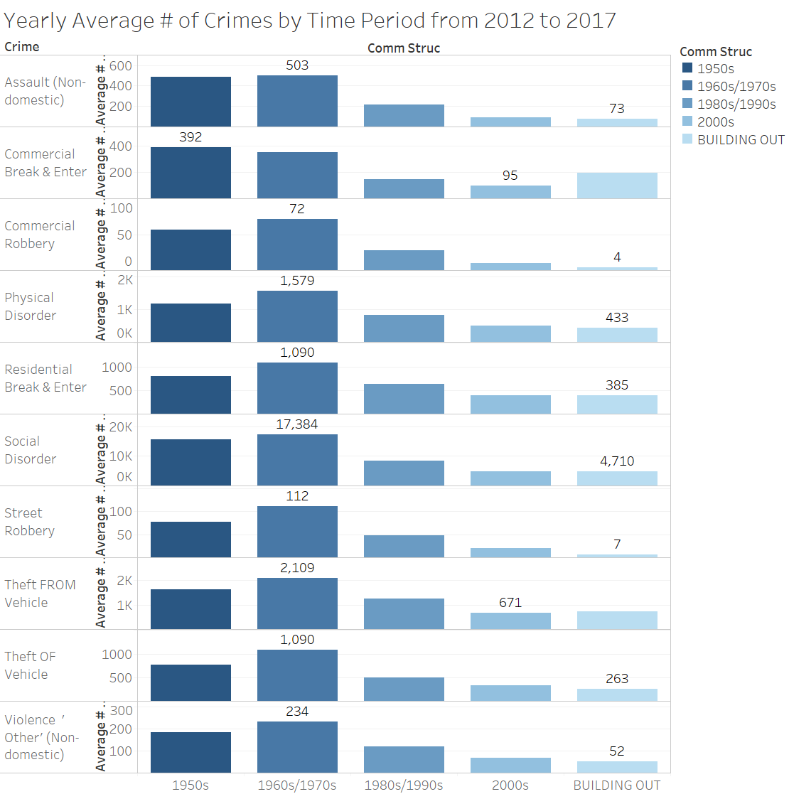
I started off by filtering out the communities that were not residential. In the Calgary shape file data set, values I included from the column COMM STRUC are 1950s, 1960s/1970s, 1980s/1990s, 2000s, and Building Out. Values that I excluded Centre City, Inner City, Employment, Other, Parks and Undeveloped, because they do not inform of what time period communities were built. In the column Class, values I included are Residential and Residential Sub, while I excluded Industrial and Major Park. I made a quick graph to illustrate the average yearly crime over the time period that these communities were built, each color representing a sector (North, South, Southeast, etc.). The yearly crime is calculated by the aggregating the sum of the crime counts (Value column) from 2012 to 2017 divided by the number of distinct Years (around 6).
Some of the limitations here is that not all communities have data from 2012 (some started in 2013), so the averages for such communities will be slightly smaller. Census data for each of the communities will also be helpful to normalize the data more but due to time contraints I was not able to integrate this. As such, the averages for sections with outliers (e.g. Forest Lawn built in the 1950s) will pull up the average a lot, since it has a much higher value than all the other communities in the same time period.
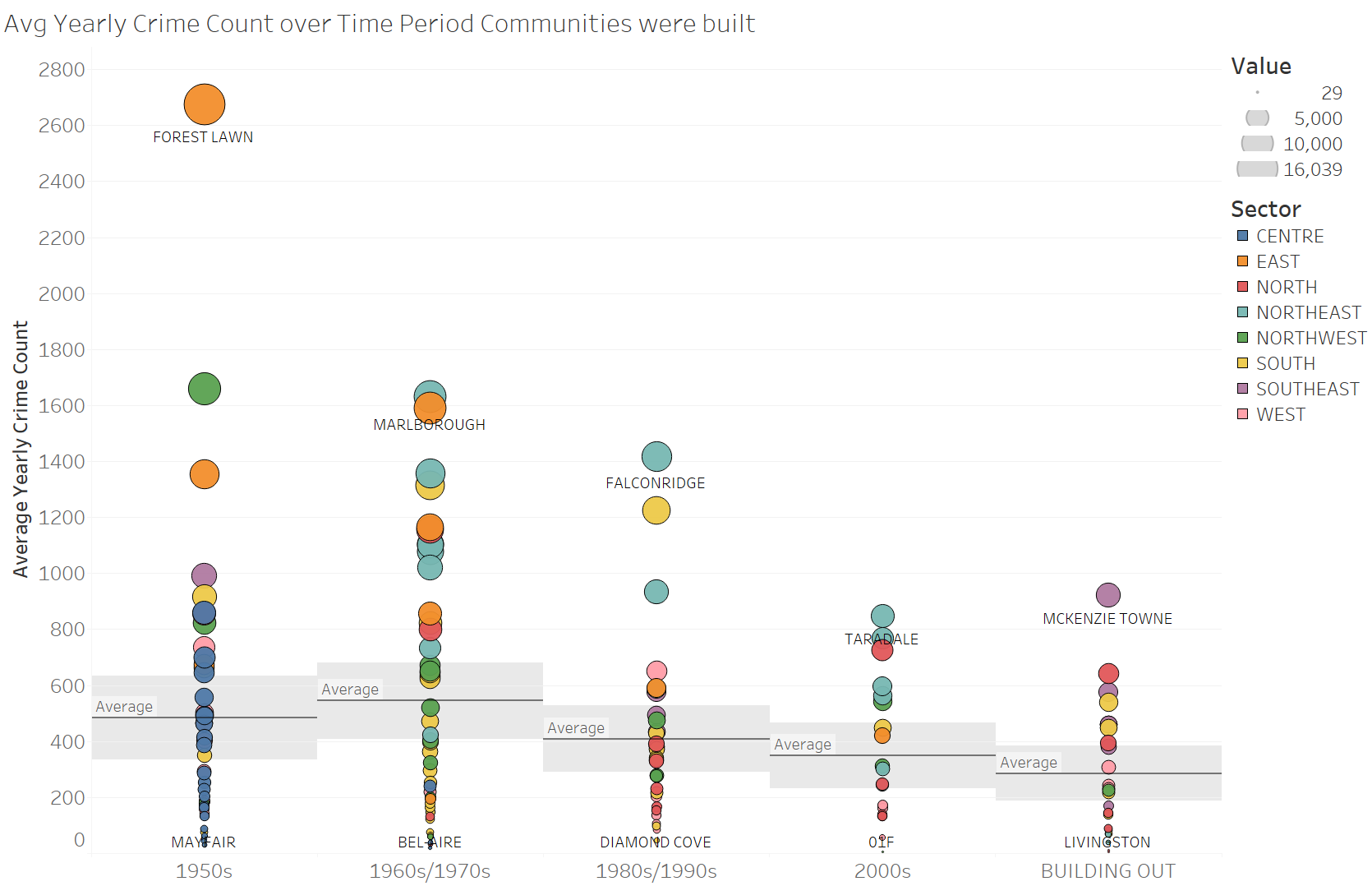
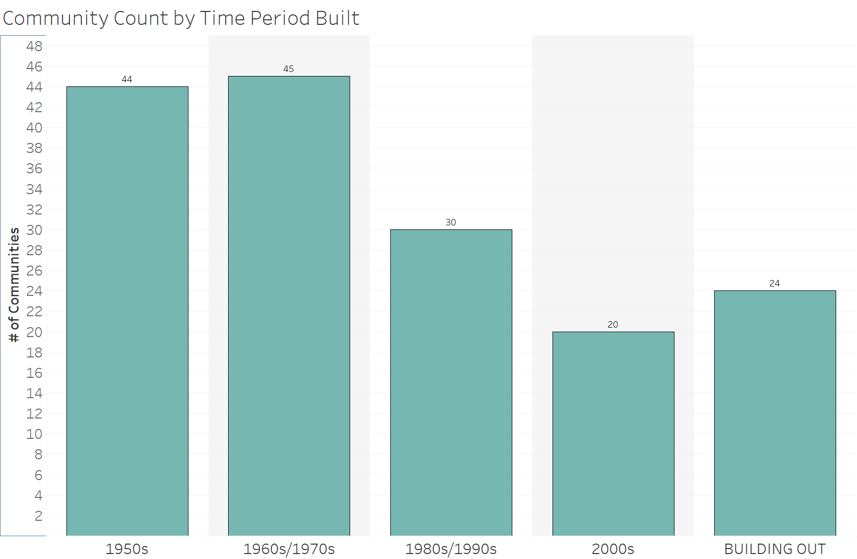
It seems that the community with the most crime in each time period that the communities were built (e.g. 1950s, 1960s/1970s, 1980s/1990s, 2000s, and Building Out) does seems to follow a downward trend of crime, the newer the community is. However when we look at the average number of crimes per time period, we see that there is a slight downward trend between 1960s and onwards, but communities in the 1950s actually have a lower average crime count than the 1960s/1970s. Looking at the averages, I wondered if the different number of communities was affecting the averages.
Breaking it off and looking at it by sector, and by time period:
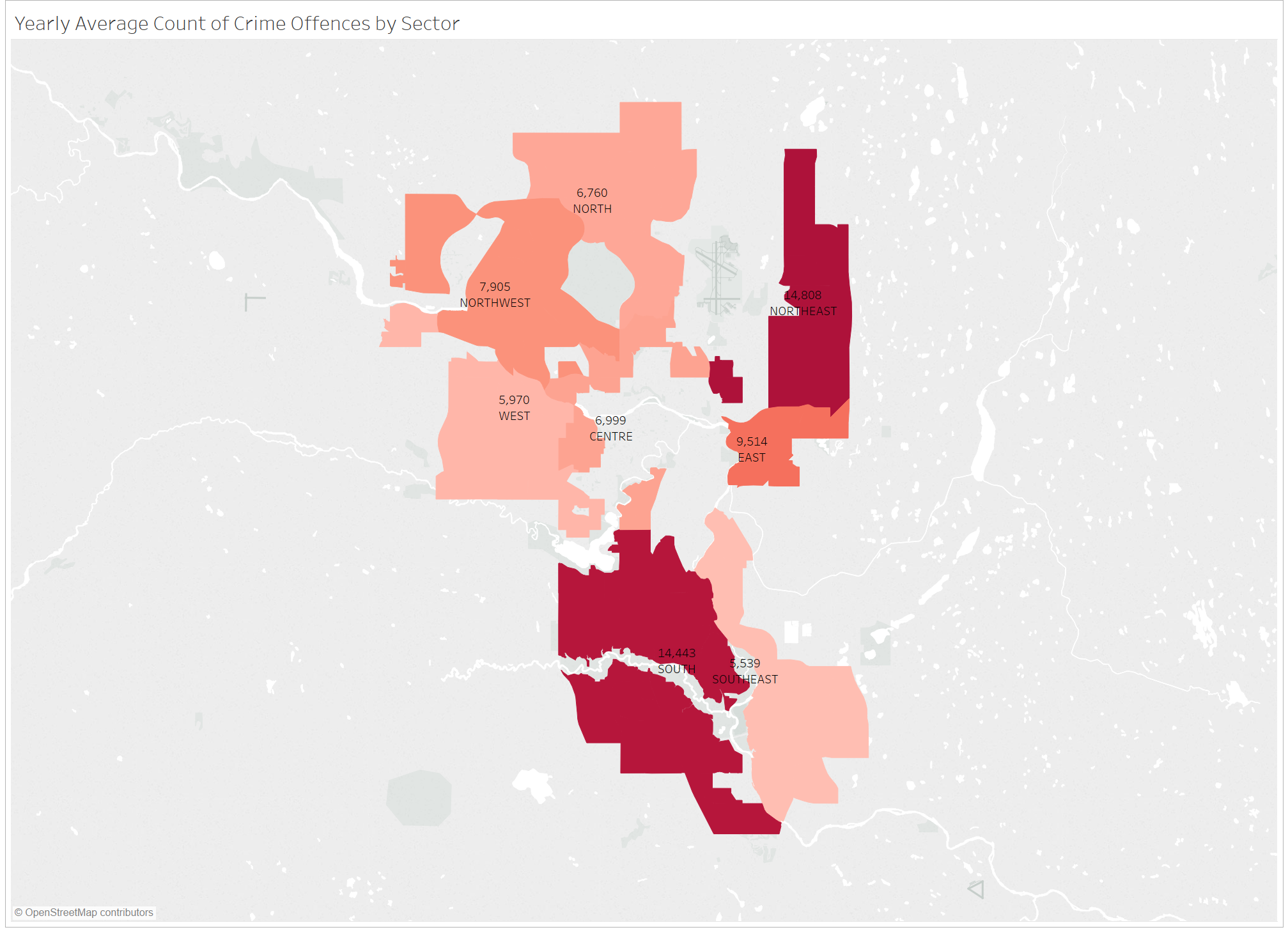
It seems like by sector, the northeast has the highest average yearly crime rate, with the south being a close second. When we split the data up by time period communities were built, and have the average yearly crime for each sector on a separate y-axis, it seems like in the 1960s/1970s there were 45 communities built, while in the 1950s there were 44. Looking at the graph below it seems like the the older communities, especially ones built in 1960s/1970s, had a higher average yearly crime count. It also looks like sectors like the northeast and south had the most overall yearly crime.
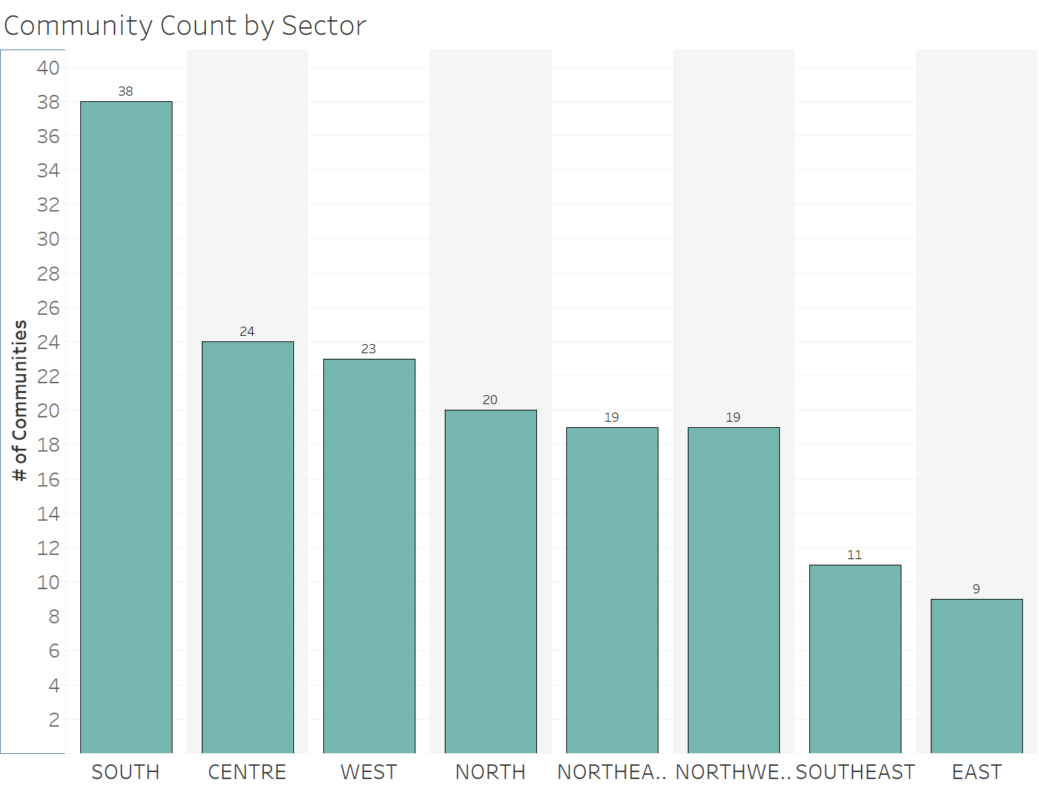
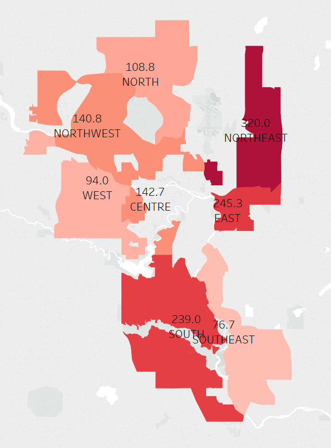
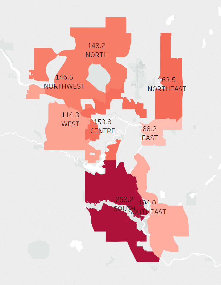
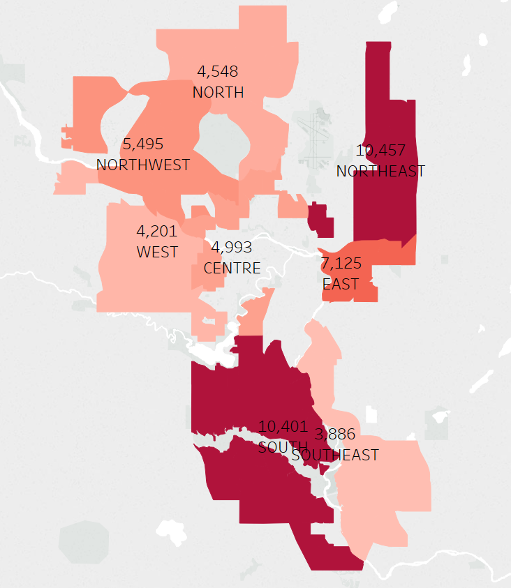
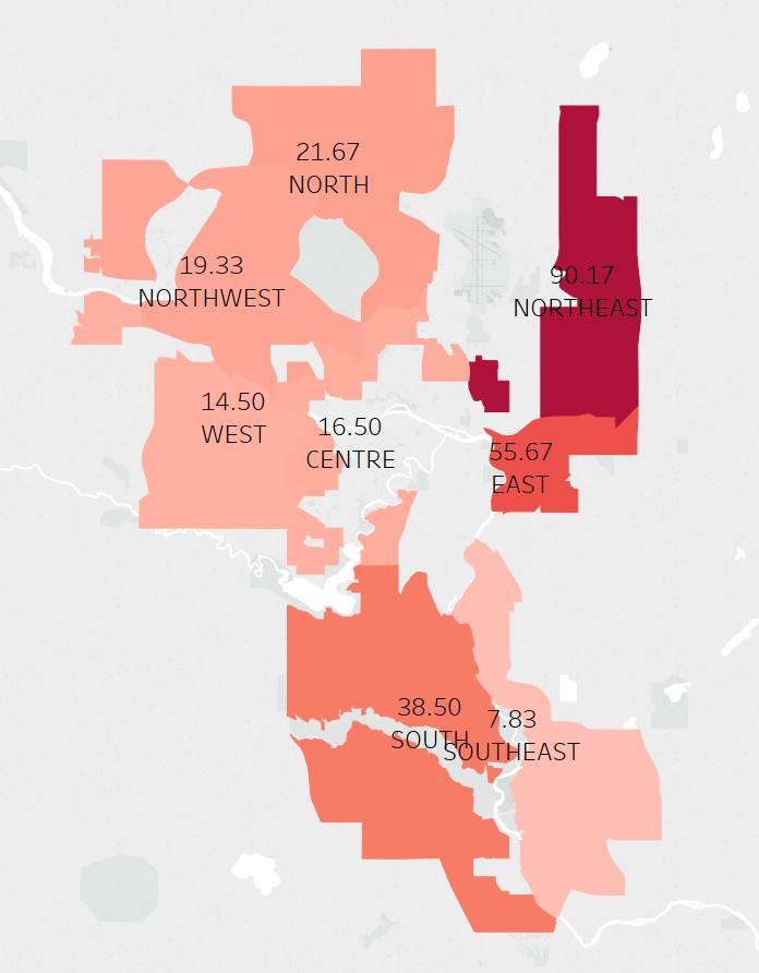
Here are some crimes by sector, still filtered with the values mentioned earlier. The Northeast and South seem to have the most crimes, but again this is expected because the south has the most residential communities. Even though the Northeast has less communities than the north and west, it still has more overall crime which is pretty interesting. Other data needs to be integrated to this data source to find out why this is the case.
Just because there are more crimes in some sectors does not necessarily mean they're bad places. This data is not normalized by community, and each community varies in population. This information may be helpful to determine how to allocate police forces depending on sectors. To summarize all the charts above, it seems that older communities may be attributed to more crime, and specific sectors such as the Northeast or South may contribute to crime as well. In the first chart, it looks like the top communities for crime per time period built come from the northeast or east sector.
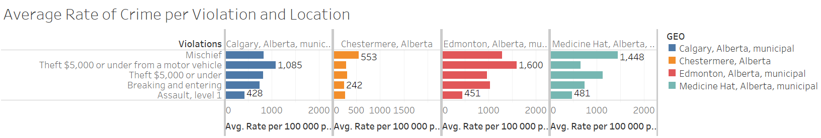
For this question I chose to filter in Calgary, Edmonton, Medicine Hat and Chestermere and filtered out Alberta, since we are interested in cities in Alberta, not Alberta itself. I did this by filtering just the top 5 results by the sum of violations and plotted them by location and averages on the column set, and violation on the row set. I filtered any value that has the term "Total" or "Other" because they are aggregations of other counts. I checked that the top 5 violations were the same for all the locations, then had the Violations values on the row set. The values were calculated by taking the average of the violations (aggregating the sum value of the violation divided by the distinct number of years).
We see that for the Calgary and Edmonton, the highest crime rates comes from Theft under $5,000 from a motor vehicle, while for smaller cities like Medicine Hat and Chestermere, the highest crime rates come from Mischief. I honestly don't know why the crime rate mischief is higher in places with smaller populations, but my hypothesis is that there is more organized crime in big cities. Organized crimes maybe steal components such as audio players or GPS systems, car parts from the cars themselves and sell them in the black market.
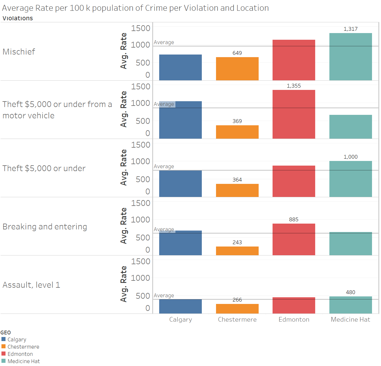
It looks like on average,across all crimes, Edmonton has consistently been above average in terms of crime rate. Calgary actually has a bigger population than Edmonton, and these rates have been normalized, so I'm not too sure why Edmonton's crime rate is consistently higher. Integration of more data sets will prove useful to see why this is the case.
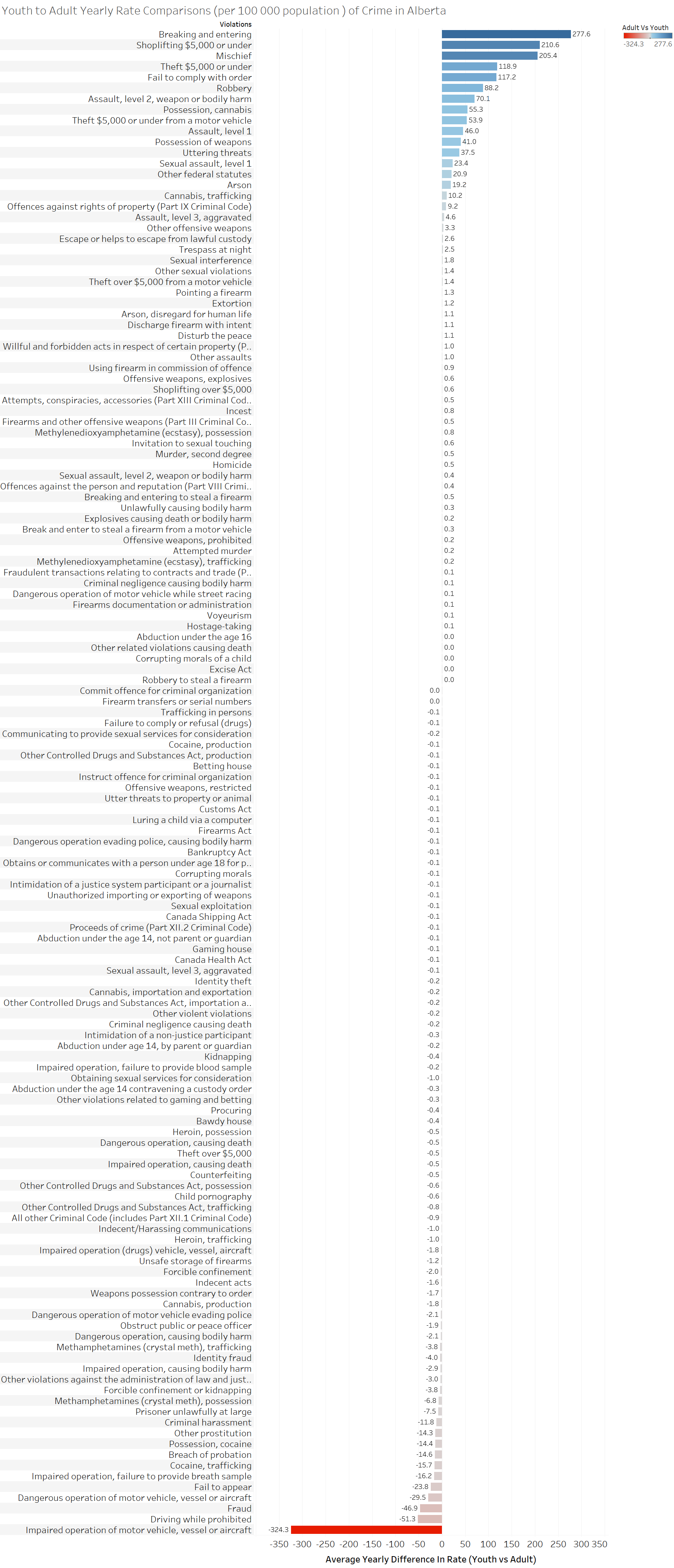
This can be done by using the augmented “By Crime” data set, with the values "Rate Youth charged per 100 000 population" subtracted with "Rate Adult charged per 100 000 population", and setting this as a new calculation field. I filtered in all values with Alberta as the location, and filtered out youth specific crimes like Youth Criminal Justice Act, since this crime was specific to youth (every time a young person from the ages 12 to 17 commits a crime they are in violation of this). I computed the yearly average difference in rate simply by subtracting the youth rate to the adult rate (youth rate - adult rate) and placed them in the bar chart. Positive values will denote a blue hue while negative values will have a red hue. Youth in this case will be all persons under 18.
Personally, the results make a lot of sense. Breaking and Entering, Shoplifting and Theft $5,000 or under would have more youth commiting these crimes maybe because of peer pressure, or to make themselves seem cooler. Not to mention youth committing these crimes probably are not so smart in the manner of executing these crimes, which makes them more likely to get caught. On the other end of the spectrum, more adults get caught driving while prohibited or impaired operation of a motor vehicle likely because not as many young people have their driver's license. Adults do more fraud related crimes likely because they know there is much more to gain from them, compared to young people's knowledge. Adults generally have more money and assets, and can probably impersonate other adults better than youth can. In gerneral it seems like petty crimes are committed more by young people, and crimes that need driver's licenses or a higher level of thinking (fraud) are committed by adults.
What are the top 2 crimes in Alberta, on a province-wide level (includes Alberta and all its cities within, such as Calgary, Chestermere, Edmonton and Medicine Hat) that are strongly correlated with one another, by year from 1998 to 2016?
For this question, I used one of my augmented data sets with the individual crimes pivoted as columns and the tool Jupyter Anaconda to calculate the correlations between all the possible crimes. Here are the commands I used:
      # imports
      import pandas as pd
      import numpy as np
      import matplotlib.pyplot as plt
      import itertools as it

      # this allows plots to appear directly in the notebook
      %matplotlib inline

      d = pd.read_excel('some_alberta_pivoted.xlsx', index_col=0) # retrieve the data
      corr=d.corr() # find correlations using built in correlation function
      corr
      ndf = pd.DataFrame([], columns=list("ABCD"))
      for c in corr.columns:
          for r in corr.index:
              df2 = pd.DataFrame([[str(c)+" , "+ str(r), corr[c][r],c, r]], columns=list("ABCD"))
              ndf = ndf.append(df2)

      ndf.to_csv("corr.csv")
I sorted the correlations in descending order and exported the results to Excel.
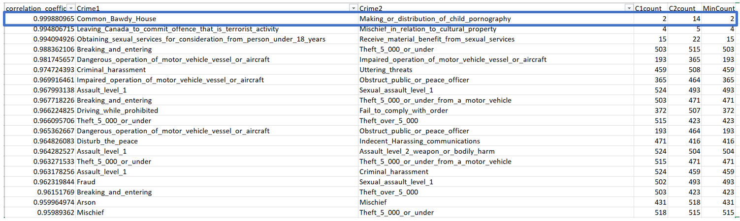
Initially, I had high hopes that the top correlation pair was actually correlated. However when I later plotted the values in a correlation chart, I found out only two data points in the chart. Confused, I did some investigation by summing up the total number occurences per crime, per year and extracted the minimum number of occurences for the pair of crimes.These counts were extracted by filtering in STAs in (Actual Incidents, Total Persons Charged, Total Adult Charged, Total Youth Charged), while filtering out the rates and the percentage change to avoid confusion. What I found was for the top correlated crimes, there were 2 counts of Common Bawdy House and 14 counts of distribution of child pornography. The next 2 had few numbers as well, 4 and 15 respectively. Considering these numbers I cannot assume these crimes are actually correlated because the number of occurences are too low.
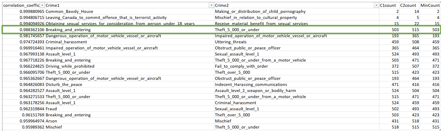
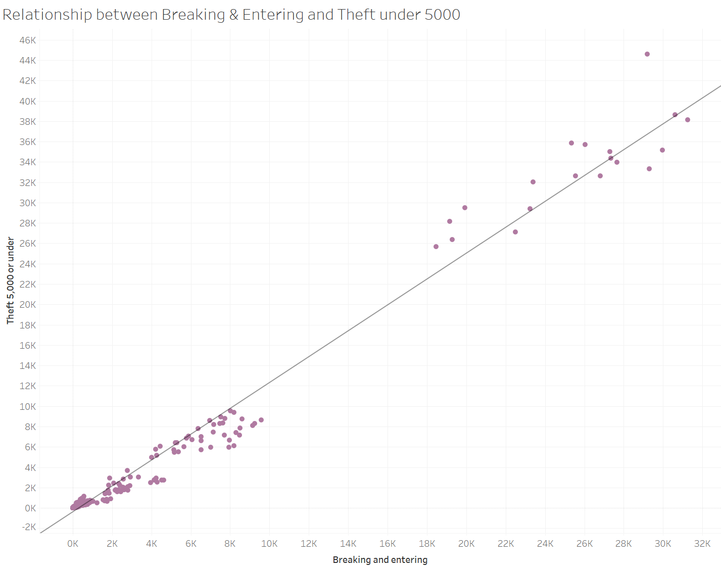
It turns out the highest pair of crimes that are most likely correlated is breaking and entering, and theft 5,000 or under. Looking at the minimum count for both these crimes, we get 500 counts which I think is a reasonably high amount. The correlation pair for me makes sense because if you are going to steal something, it most likely is in a building of some sort that you have to break and enter to. My hypothesis is, based on what we saw earlier more youth commit break and enter crimes, thus most likely don't have access to cars which means that tha value of the things that they steal are most likely things that need to be carried on foot. Another assumption that I have is that a lot of individual things in a house don't actually cost more than $5,000. If they do, it's likely that they can't be easily stolen.
This is the code used for multiple regression:
import statsmodels.formula.api as smf
                lm_crime = smf.ols(formula='Murder_first_degree ~  '\
                '+Infanticide'  \
                '+Commit_offence_for_criminal_organization'  \
                '+Advertising_sexual_services'  \
                '+Methamphetamines_crystal_meth_importation_and_exportation'  \
                '+Cannabis_importation_and_exportation'  \
                '+Heroin_importation_and_exportation'  \
                '+Methylenedioxyamphetamine_ecstasy_possession'  \
                '+Competition_Act'  \
                '+Hoax_terrorism'  \
                '+Abduction_under_the_age_14_not_parent_or_guardian'  \
                '+Advocating_genocide'  \
                '+Cocaine_importation_and_exportation'  \
                '+Dangerous_operation_evading_police_causing_death'  \
                '+Instruct_offence_for_criminal_organization'  \
                '+Explosives_causing_death_or_bodily_harm'  \
                '+Break_and_enter_to_steal_a_firearm_from_a_motor_vehicle'  \
                '+Criminal_negligence_causing_death'  \
                '+Methylenedioxyamphetamine_ecstasy_trafficking'  \
                '+Commission_or_instructing_to_carry_out_terrorist_activity'  \
                '+Altering_removing_or_destroying_Vehicle_Identification_Number_VIN'  \
                '+Dangerous_operation_causing_death_while_street_racing'  \
                '+Conspire_to_commit_murder'  \
                '+Firearm_transfers_or_serial_numbers'  \
                '+Cocaine_production'  \
                '+Abduction_under_the_age_14_contravening_a_custody_order'  \
                '+Dangerous_operation_causing_death'  \
                '+Heroin_trafficking'  \
                '+Communicating_to_provide_sexual_services_for_consideration'  \
                '+Facilitate_terrorist_activity'  \
                '+Leaving_Canada_to_commit_offence_that_is_terrorist_activity'  \
                '+Manslaughter'  \
                '+Impaired_operation_drugs_causing_death'  \
                '+Breaking_and_entering_to_steal_a_firearm'  \
                '+Invitation_to_sexual_touching'  \
                '+Cannabis_production'  \
                '+Bankruptcy_Act'  \
                '+Methamphetamines_crystal_meth_trafficking'  \
                '+Kidnapping'  \
                '+Luring_a_child_via_a_computer'  \
                '+Arson_disregard_for_human_life'  \
                '+Indecent_acts'  \
                '+Assault_level_3_aggravated'  \
                '+Attempted_murder'  \
                '+Arson+Extortion'  \
                '+Homicide'  \
                  , data=d).fit()

                # print the coefficients
                print(lm_crime.params)
                lm_crime.summary()
And this is the output:
Intercept                                                            0.180462
                    Infanticide                                                         -0.232313
                    Commit_offence_for_criminal_organization                             0.209033
                    Advertising_sexual_services                                          0.164596
                    Methamphetamines_crystal_meth_importation_and_exportation            0.612533
                    Cannabis_importation_and_exportation                                -0.110311
                    Heroin_importation_and_exportation                                  -0.000869
                    Methylenedioxyamphetamine_ecstasy_possession                        -0.249338
                    Competition_Act                                                     -0.030225
                    Hoax_terrorism                                                       0.310415
                    Abduction_under_the_age_14_not_parent_or_guardian                   -0.059490
                    Advocating_genocide                                                  0.463646
                    Cocaine_importation_and_exportation                                 -0.094991
                    Dangerous_operation_evading_police_causing_death                     0.157164
                    Instruct_offence_for_criminal_organization                           0.500772
                    Criminal_negligence_causing_death                                    0.003857
                    Methylenedioxyamphetamine_ecstasy_trafficking                        0.027840
                    Commission_or_instructing_to_carry_out_terrorist_activity           -0.077850
                    Altering_removing_or_destroying_Vehicle_Identification_Number_VIN    0.060641
                    Dangerous_operation_causing_death_while_street_racing                0.173869
                    Conspire_to_commit_murder                                           -0.213716
                    Firearm_transfers_or_serial_numbers                                 -0.121448
                    Cocaine_production                                                   0.157958
                    Abduction_under_the_age_14_contravening_a_custody_order              0.000255
                    Dangerous_operation_causing_death                                    0.060452
                    Heroin_trafficking                                                  -0.093765
                    Communicating_to_provide_sexual_services_for_consideration          -0.076533
                    Facilitate_terrorist_activity                                       -0.117903
                    Leaving_Canada_to_commit_offence_that_is_terrorist_activity          0.908075
                    Manslaughter                                                        -0.049829
                    Impaired_operation_drugs_causing_death                               0.315761
                    Breaking_and_entering_to_steal_a_firearm                            -0.026077
                    Invitation_to_sexual_touching                                        0.103762
                    Cannabis_production                                                 -0.025856
                    Bankruptcy_Act                                                       0.256307
                    Methamphetamines_crystal_meth_trafficking                           -0.019289
                    Kidnapping                                                           0.107383
                    Luring_a_child_via_a_computer                                        0.337560
                    Arson_disregard_for_human_life                                       0.205432
                    Indecent_acts                                                       -0.051292
                    Assault_level_3_aggravated                                          -0.081662
                    Attempted_murder                                                     0.128292
                    Arson                                                                0.013254
                    Extortion                                                            0.073964
                    Homicide                                                             0.730581
                    dtype: float64
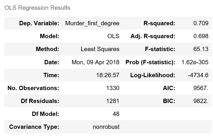
The best r-squared value that I could come up with for this is 0.709. I first dumped all the crime columnms in the model and checked to see which p-values were more than 0.05. There are still some values here that have a value of less than 0.05, but I kept them because removing them dropped the r-squared significantly. The strongest coefficient related to first degree murder is homicide as shown below.
All the values that are above 0.05 have significant p-values, whereas all the values below that do not. Thus for all the crimes with significant p-values we might reject the null hypothesis (that there is no association between those features and first degree murder), and fail to reject the null hypothesis for all values below 0.05. Values such as Homicide, Crytal Meth importation and exportation, and all values that are positive are all positively associated with first degree murder, whereas Infanticide is negatively associated with First Degree Murder.
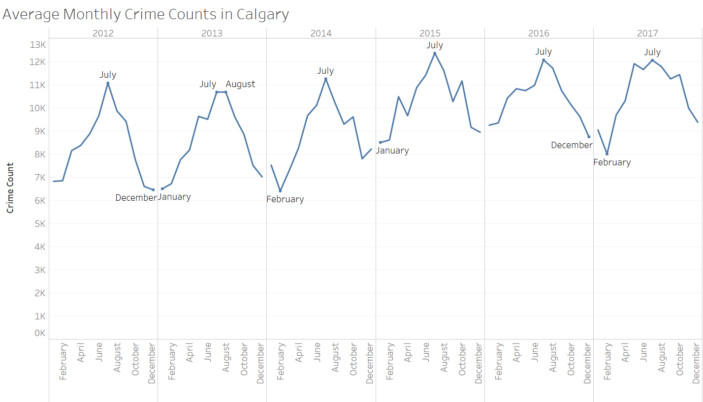
My process for this question was pretty straightforward: I plotted the months along the x-axis (column list) and the average value for each month along the y-axis (row set). The averages were done by taking the sum of the values divided by the number of distinct years, which in this case is 18 (1998- 2016), and is further separated into averages for each month from the column list.
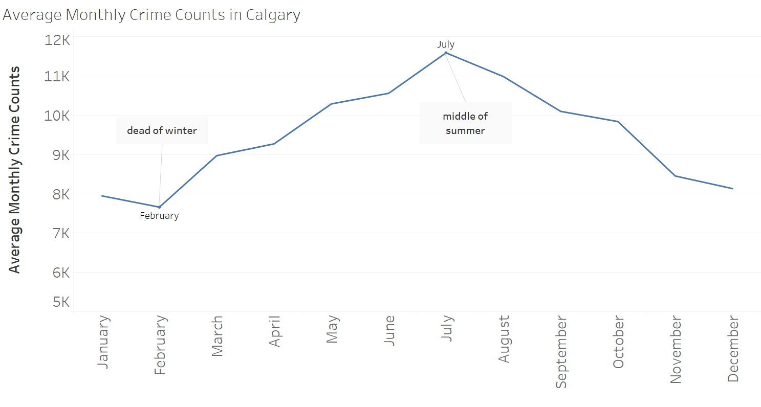
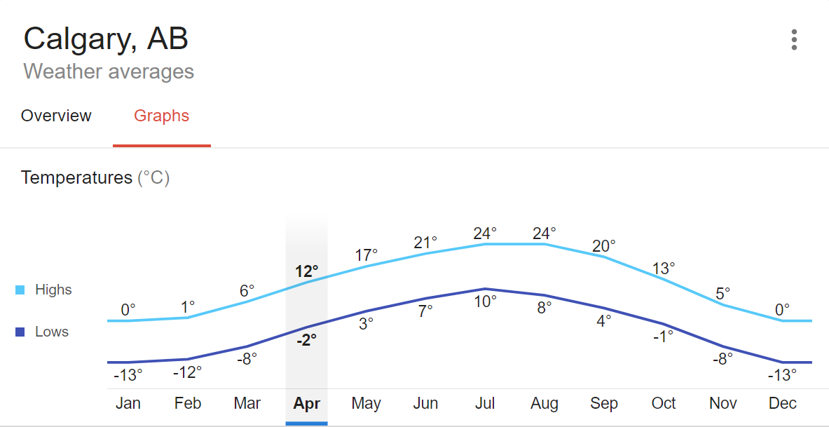
It looks like the peak of crime in Calgary is found in July, and the lowest point is found in February. Doing a quick Google Search for average temperatures by month in Calgary, we can see the curvature of the lines in both graphs look very similar, and there's reason to believe that the crime rates might be correlated with temperature.
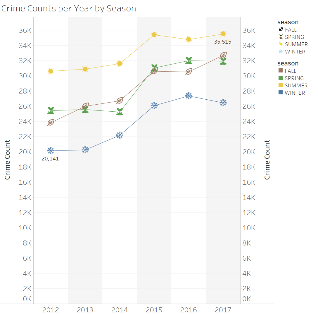
The following seasons (in Canada) are made up of the following months:

                Spring is from March to May
                Summer is from June to August
                Fall is from September to November
                Winter is from December to February
It looks like over the years crime in Calgary has had a cyclical pattern, with summer having the most crime each year and winter having the least crime. Personally this makes sense because Calgary winters are very cold and you would not want to stay out for a long period of time.
How do the crime rates involving drugs such as cocaine and cannabis differ across Calgary, Edmonton and Medicine Hat over the years?
What I did for this analysis question was filter the values "Total cannabis, trafficking, production, or distribution" and "Total cocaine, trafficking, production, or distribution", and further filtered the locations to be Calgary, Edmonton and Medicine Hat. Using the rater per 100 000 population column, I plotted the values by year from 1998 to 2016, each row denoting a location (Calgary, Edmonton, Medicine Hat).
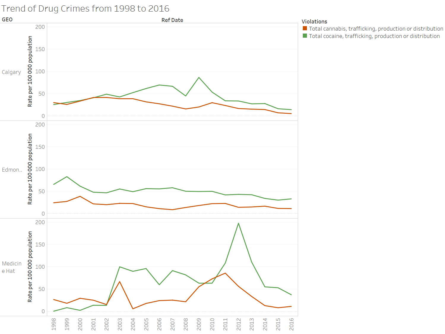
There is a noticeable spike for Calgary in 2009, and 2012 in Edmonton for total counts of violations pertaining to cocaine, and I think these years when the police do drug busts, they catch multiple people at a time associated with the drug ring. There's also noticeable spikes for cannabis in 2002 and 2011 for Medicine Hat.
For the graph below I changed things up a bit so I can see a direct comparison between the municipalities for each year, so I had the column list as the year and location, and the rows to be the specific type of violation and the rate of that particular crime per 100 000 population.
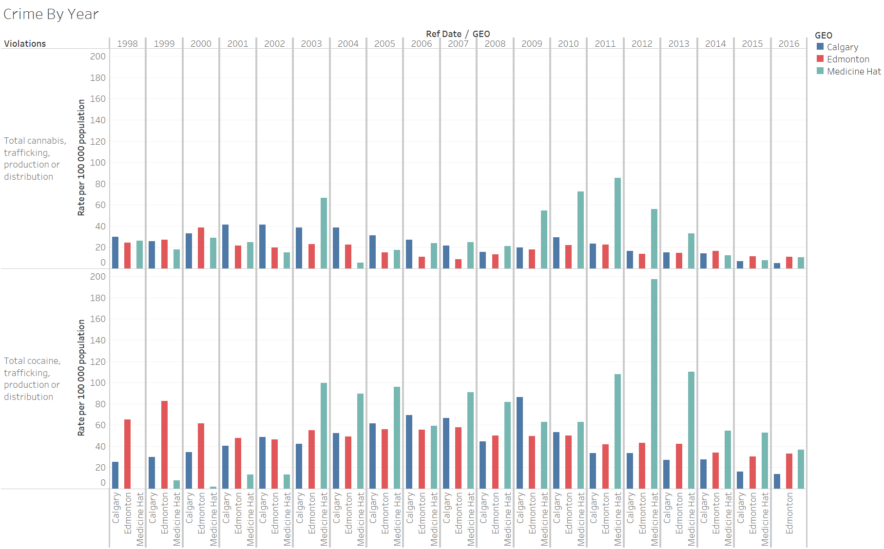
I wanted to see a direct comparison Based on the visualizations above, I wondered why Medicine Hat's average was so high. After some digging it turns out that the population of Medicine Hat is less than 100 000 people. I'm not entirely sure how Stats Canada did the normalization of rates but my suspicion is that this might skew the results up for Medicine Hat. In summary it looks like comparing all three cities, for cannabis from 1998 to 2006 it was mostly Calgary that had the most crimes, then Medicine Hat dominated the scene from 2007 to 2013. From there the rates significantly dropped between 2014 to 2016. For cocaine, Edmonton has a lot more crimes from 1998 to 2000, then from 2003 to 2016 Medicine Hat mostly more crimes compared to the other two cities. I noticed that there is a drop in these crimes in recent years, across all three cities, from 2014 onwards. Maybe this is because organizations involving crime are becoming a lot smarter and more discreet in how they traffic, produce or distribute these drugs? Or maybe there is more stigma against doing drugs, and governments are more proactive in advocating against drugs during this time? I also noticed that there is a dip in cannabis crimes between 2005 to 2008, interesting but I have no hypothesis as to why. Perhaps it was simply just a more peaceful time during that period.